Genetic Color Space Transform Optimization Algorithm.

Premise:

The benefits of accurate and consistent color space conversions from camera space to delivery space are well discussed. Sadly some camera spaces (eg DJI D-Log-M) are undocumented and there is no good method for this.

Linear tone curves mean an image shot at 0 EV, and same image captured at +1 EV, every pixel should have double the RGB values. I explored this principle here (https://www.zebgardner.com/photo-and-video-editing/dji-d-log-m-colorgrading) to try and manually build a CST that converts D-Log-M to linear.

The same chart was shot at 10 different exposures, the shutter time moved one stop between each. If a correct log to lin tone curve is applied, the shot at -3EV, raised 3 stops in edit should match the 0EV shot. So a custom tone curve was manually adjusted to try and best satisfy this for all 10 shots.

The second part to as CST is mapping the camera color primaries to your intended space. Doing this manually is not difficult but certianly leaves a lot of accuracy to be desired. Manually created hue-hue and hue-sat curves to map the 6 color chips of the 0EV shot to the correct spots on the vector scope. This can't correct for any color difference in the -3EV shot as you now have a 3-dimensional color problem and only various 1-d curves to try and correct this.

My goal was to create a program that can take in multiple exposures of a test chart and mathematically perform the similar linear mapping. And also evaluate the color portions over the various shots to produce the most accurate colors as well.

Davinchi Resolve has and automatic color checker tool. But it is famously quite bad; https://forum.blackmagicdesign.com/viewtopic.php?f=21&t=176392&hilit=+checker

I don't know the details that Black Magic use for it. But since it runs quite fast, I suspect it does something like linear regression to produce a 3x3 matrix for the color primaries mapping. And maybe a similar logarithmic fit for tone curve mapping. The log fit would explain why fails so often, if the camera tone curve isn't actually logarithmic.

Also this tool only works on a single frame, and the tone chips of charts only cover about 5 stops of range. And are certainly no where near black/white point of the sensors (12+ stops).

Math:

I did experiment with trying to perform regression fits to make a direct tone mapping and produce a closed form equation as the result. This would have the advantage of being very fast to compute the regression. And produce a (relatively) simple formula that could be put into a DCTL to give precise mathematical conversions in resolve. A 3x3 Matrix could then similarly be calculated for the color primaries.

But I discovered that d-log-m does not have a good logarithmic mapping to linear space. No doubt a problem for other camera spaces as well. And curve fitting algorithms need to know the basic 'shape' of the curve they are trying to fit to, and then tweak the parameters to minimize there error to that curve.

So I decided to ultimately produce a 3d lut as the CST device. These work by having a list of input RGB values that get mapped to new output RGB values, and any number that isn't in the table is interpolated between. This has the flexibility to be basically any arbitrary mapping that you don't necessarily have a formula to describe.

So how to produce this lut?

Color chart manufacturers publish the expected LAB values for the color chips on their charts. LAB space is convenient in that L is the luminance values and A & B describe the color.

https://en.wikipedia.org/wiki/CIELAB_color_space

So we can calculate how far away the L values are in our captured image are away from the published L values for the charts. We then adjust the tone curve in our conversion to minimize this error. 'Adjust' is a big word there though. If we have 6 different exposures for our test charts, and each chart has 12 tone chips, how do we know where in our tone curve to adjust, what way, and how much?

Answer, guess randomly. https://en.wikipedia.org/wiki/Genetic_algorithm

Thousands of kids:

If we had a tone curve of 10 points, and we wanted to test each of those 10 points with 8 different values, that would be 10^8 test cases, 100 million. And 8 different values really isn't anywhere near the resolution you would need to get an accurate curve.

So instead we randomly adjust each of those 10 points an amount. We then calculate the error for our 6 exposures for the 12 tone chips. If the error is better than it was before we made a good adjustment. Try 1000 different random adjustments and keep the best of the 1000.

This best from that generation will be the parent for a new set of 1000 new random guesses the next time. Since our PC has multiple cores, lets instead have 12 parents, take the best child from each of those. Pair them up, average them and use them as the new parents.

This means we don't need to do the 100 million tests to exhaustively search all possible tone curves for the best one. We instead can get a very good result in only about 5 generations. So 5 x 12 x 1000 x 10, 600 thousand guesses.

Enter the Matrix:

With an accurate tone curve we can work on color. A 3x3 matrix is the classical way to convert color primaries. And only 9 variables, they make it simple for our above algorithm.

https://filmmakingelements.com/what-is-a-3x3-matrix-in-color-grading/

We apply the tone curve to our input images, apply a unity 3x3 matrix and calculate the A & B errors from where the test chart says we should be. Perturb each of the 9 values in the matrix and compute the errors again. Run this through the same genetic algorithm and I found this converges to a quite accurate solution in only 3 generations of 500 children each.

With the tone curve and a 3x3 matrix we have everything we need for a CST. I however found in practice the results were not very good.

The 3x3 has no concept of luminance. If the mids need more green, the shadows and highlights are getting more green too. And I found, at least on the d-log-m curve I was experimenting on it had a horrible green cast to the highlights.

More Curves:

So why not repeat the tone curve we did in step one, but instead have it create a mapping of how much green should be in the image for the shadows, mids, highlights. And obviously for Red a Blue as well. And don't limit it to just 3 control points, give it 10 to control again. And we measure the color error in the image as we adjust these 10 control points in these 3 independent curves. Again tweaking the 10 points to produce the least error in all 6 different test shots.

This allows us to correct for color cast from different tones but it doesn't let you control saturation across the tones. A red apple becomes more saturated when you increase the red and reduce the green and blue. With 3 individual 1-d curves you can't adjust saturation as the curves need to interact with one another.

Cubes:

This is where color cubes come in. Cubes can do everything we did with 1d curves and 3x3 matrix, why not start there? If you have opened a 65-cube lut file you see 274 thousand rows with a R G and B value for each. So not instead of trying to guess good values for our 10 points on a tone curve we have 274x3 thousand to choose from and need to try and pick the right ones to adjust and by how much.

So the 1d tone curve, 3x3 matrix and 3x 1-d color curves are really to build a color cube that is pretty good and we can then start to refine it. And we also aren't going to work on a 65-cube with 822k entries, so lets do a 10-cube with 3k points instead

We apply this cube conversion to our 6 exposures and calculate the errors for each of the 24 chips on each chart. Rank them by the worst error. We find which of the 3k points in the cube is controlling that chip and perturb it. Then calculate the error for all 6x24 chips. If we made the error better, good keep that change, if we made it worse, revert the change. Go on to the next worst error chip in the 144. Loop through the worst 20% of the chips and start again at the top to see if you can do better.

More Children:

This method of targeting the worst chips I was expecting to produce a significant improvement in the errors of the worst chips. It ultimately didn't. The algorithm also can't really be multi-threaded (that I know of) since you are testing changes to each chip individually and you can't test the next until you found the 'best' solution for the first. So its slow to execute.

The genetic algorithms we used initially are great in that we can spin of 12 threads to each try 1000 children and then report back their individual best results. We average those together and keep the 12 good results and send them off again for another generation. So it can run very fast due to parallelism.

So lets do that to the cube. Spin up 12 parents. Have them make 200 kids which each take one of the 1000 RGB points in the cube. Perturb it and calculate the error. Report back the results and go again for another 10 generations.

At the end we should have a cube that very accurately maps the 6 test charts linear space. We can then go from there easily to Davinchi Wide Gammut to edit or Rec.709 for delivery.

Results:

These exact numbers are pretty meaningless, and using a different camera will no doubt produce different numbers. But I do think the reader may find interest in the progression of how the average error is reduced as the algorithms are run.

The program applies our hopeful linear conversion, adjusts gain on over/under exposed charts and then converts to LAB space to calculate the error vs the manufacture specs for the chart.

I dump that average error to the console as it is run to gauge progress.

The first step is only L error, ignoring A and B. Using the rec-709 to linear formula as our starting assumption of what our actual conversion would be we get a average luma error of 8.7

After the first generation this error is 5.3, and after five generations it is 3.9.

The 3x3 matrix initial assumption is the unity matrix (no change). The A & B error average is 5.2. After one generation 4.70, three generations 4.68.

The R, G, B 1-d curve optimization is run next, again only concerned with A & B error, starts at the 4.68 error the 3x3 matrix left us with. One generation, 4.61, three generations 4.55. We can also calculate the combined LAB error and it finished at 4.4

Since the changes to color will affect the luminance of the color chips, somewhat, our initial assumption of luminance curve has changed. The Luma error is now 3.65. So this whole 3 step process is repeated five times.

Final Luma error is 3.24, Color error 2.95. With LAB combined error 3.55. So a 24% improvement over round 1.

Converting from the 1d curves and 3x3 to a 3d cube is not a 1 to 1 mapping. The LAB error after conversion is 3.58.

Running the genetic algorithm on the cube for 15 generations results in LAB error of 3.42

Running the algorithm that targets just the chips with most error one at a time run through 10 loops on the worst 20% of chips reduces the error to 3.41 (So it probably isn't worth the CPU time)

Running the genetic algorithm again for 15 generations reduces error to 3.31. This is the final model that was converted to a 65-Cube lut and used in Resolve for the test results at the end.

Discussion:

Over-fitting:

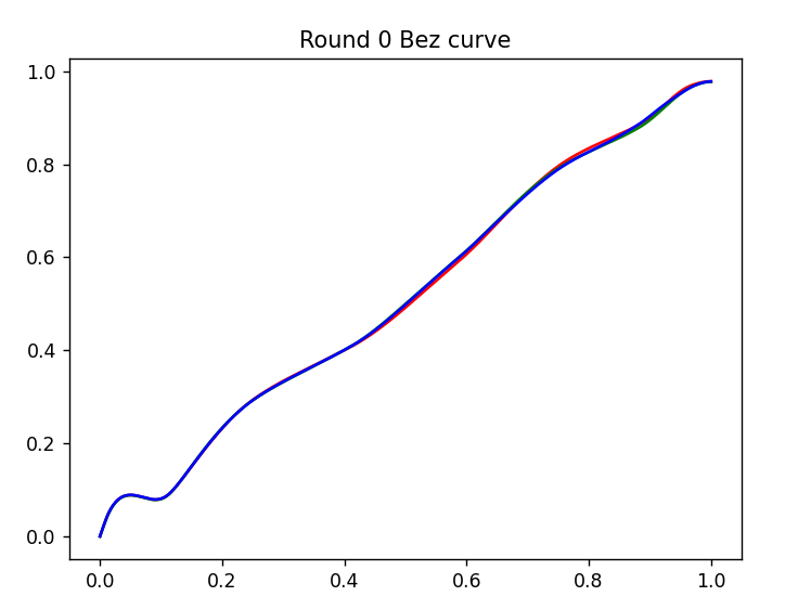
Over-fitting is the primary concern. The following shows and extreme example where 30 control points are used for the luma curve fit. The algorim may produce a low average error, but this will no doubt result in a horrible image

This is the same parameters, but instead of 30 control points, 10 are used. This smooth curve is probably going to produce a more accurate final image.

Interpolation method.

Our goal should be to produce a final correction curve that smoothly transitions between values, as discussed in the over-fitting section, wild swings may produce a lower error calc, but not likely to produce a better real image.

Interpolation methods have a big impact on this. They also have a significant impact on execution speed. Linear interpolation and Nearest will execute very fast, but will produce sharp transitions and stair steps in the resulting curve. Cubic interpolation forces a smooth curve, but I found it often produced unwanted ringing/overshoot. Makima interpolation seemed to be the best solution, it is not particularly fast to execute, but it doesn't overshoot, and produces smooth transitions.

https://blogs.mathworks.com/cleve/2019/04/29/makima-piecewise-cubic-interpolation/

This method doesn't appear to be an option for the 3d interpolation needed for the 3d cube (at least in python). Pchip looks to minimize overshoot, but was very slow to execute. Cubic was ultimately chosen as it was acceptable execution speed and should produce smooth transitions. I I don't know how to visualize overshoot in the 3d cube, so we will just pretend it doesn't happen.

Local Minima.

The algorithm if fundamentally doing gradient assent. If a change produces lower error, it takes it. This doesn't guarantee that you actually found the best solution, you could just be circling around an ok solution. Bad starting assumptions will make this even more likely you never get to the best solution.

I tried to increase the probability of jumping out of a local minima in a few ways. The random guesses use Gaussian distribution. So you have a 5% chance you will get a guess that is 3 std-dev out, so maybe that wild-a guess jumps you out of the local minima. But you can't have every guess be wild as you will go in crazy directions constantly and never get to any minima.

I set the 0th child to make guesses 5x larger than all the others. So maybe it has better odds of jumping out of the minima, and using that to feed the next generation something they can refine.

Limited input data.

I am currently using a X-rite pocket video chart. It has 12 grayscale chips, the 6 primary color chips and 6 skin tones.

So the algorithm has no data on 'orange' to fit to as the chart doesn't have an orange chip. I have since got an Color-Checker SG chart with 140 chips, so a significantly larger variety of hue and saturation. But something like very saturated yellow of a sunset is something you can never replicate on a reflective chart.

White balance.

If the source images are not correctly white balanced (eg too yellow), the algorithm is going try and counter this (add blue) in the final CST. This is not desired as we would not want a CST to push every image blue.

I experimented with ways to try and remove this bias from the results, but nothing was effective. Ultimately the images captured must have correct WB in camera before sent to algorithm.

Test chart lighting.

I lit my test charts with sunlight. If poor quality (low CRI) light is used, I would expect the algorithm would push excessive saturation into colors where the light spectrum is lacking.

Exposure.

Similarly to WB, of the image the algorithm is told is 0 Ev is not actually 0 EV, it will push its results to compensate. This is a lot harder to prevent as a camera the manufacture has not documented the color space for, they have probably not specified what IRE neutral gray should be when shooting.

This ultimately ended up being guess and check for me. I assumed a certain shot was about right and checked the LAB values of neutral gray chip in the image to see if it was close the manufacture spec. And adjust exposure in camera to compensate.

For 'real' log color spaces that have a significant toe, you will expect the uncorrected image to be much brighter than final, so this will not work. I suspect you will need to apply the final CST to an image and see if it 'looks' like it is pushing exposure, and correct for what you tell the algorithm is 0 EV.

I again experimented with forcing the algorithm to not shift exposure. But never found something effective.

Lut values >1.

Along with exposure, if the algorithm is told an image is 0 EV but it is actually -1 EV, the results in the final lut will be 2x what they would have been otherwise. So values will no doubt be larger than 1.

It doesn't appear that resolve has a problem with this and a specification I found for 3d cube luts said >1 is valid.

I have considered different routes, scale results or soft clip.

If the algorithm produces a max value of 1.25 it thinks in necessary to accurately convert the image to linear, divide all the numbers by 1.25 before writing them to the lut. This would produce a slight exposure reduction from what it thought 0 EV is.

Soft clip, leave values from 0 to 0.75 unchanged and gently scale down the values above this to fit less than 1. This would leave general exposure unchanged, but I am unsure if it will produce 'weirdness' from very saturated colors where only one channel is reduced.

Or do nothing. If editing software doesn't error on >1, colorist can adjust gain if they want. Or maybe the highlights should get clipped.

Exposure in camera for the source images fed to the algorithm could be increased so that resultant calculated conversion lut is <1

Color coordinate systems for curves.

I have done all the curves in RGB space. The final cube lut needs to be in RGB space, so that makes that trivial.

If you look at the chart calibrations done with automatic tools in Light Room, they look to use the HSL (Hue Sat Lum) sliders. Also, the workflow for manually correcting an image to 6 color chips on a vector-scope is with hue-hue and hue-sat curves.

I have considered if more efficient mapping could be made by using a Hue-Hue and Sat-Sat curve instead of the 3x 1d curve I used.

A similar question could be asked if the 3d cube optimization should be done in an HSL coordinate system instead of RGB. The HSL cube would of course need to be converted back to RGB coordinates for the Lut export.

HSL space is certainly more intuitive to a human, we can say the reds need to be more saturated, or the blue should be rotated to be more green. But I am not sure this would be of any use to the algorithm I am using that doesn't have any understanding of the source of the error or how to reduce them, it only making random guesses and testing the results.

There could also be the question of if HSL to RGB conversion would make the 'smoothness' of the curve fits better or worse. If a 10 point HSL cube could produce equal error to a 20 point RGB cube, it would no doubt be a more smooth fit. But the opposite may also be true.

Further experimentation is needed.

Image results:

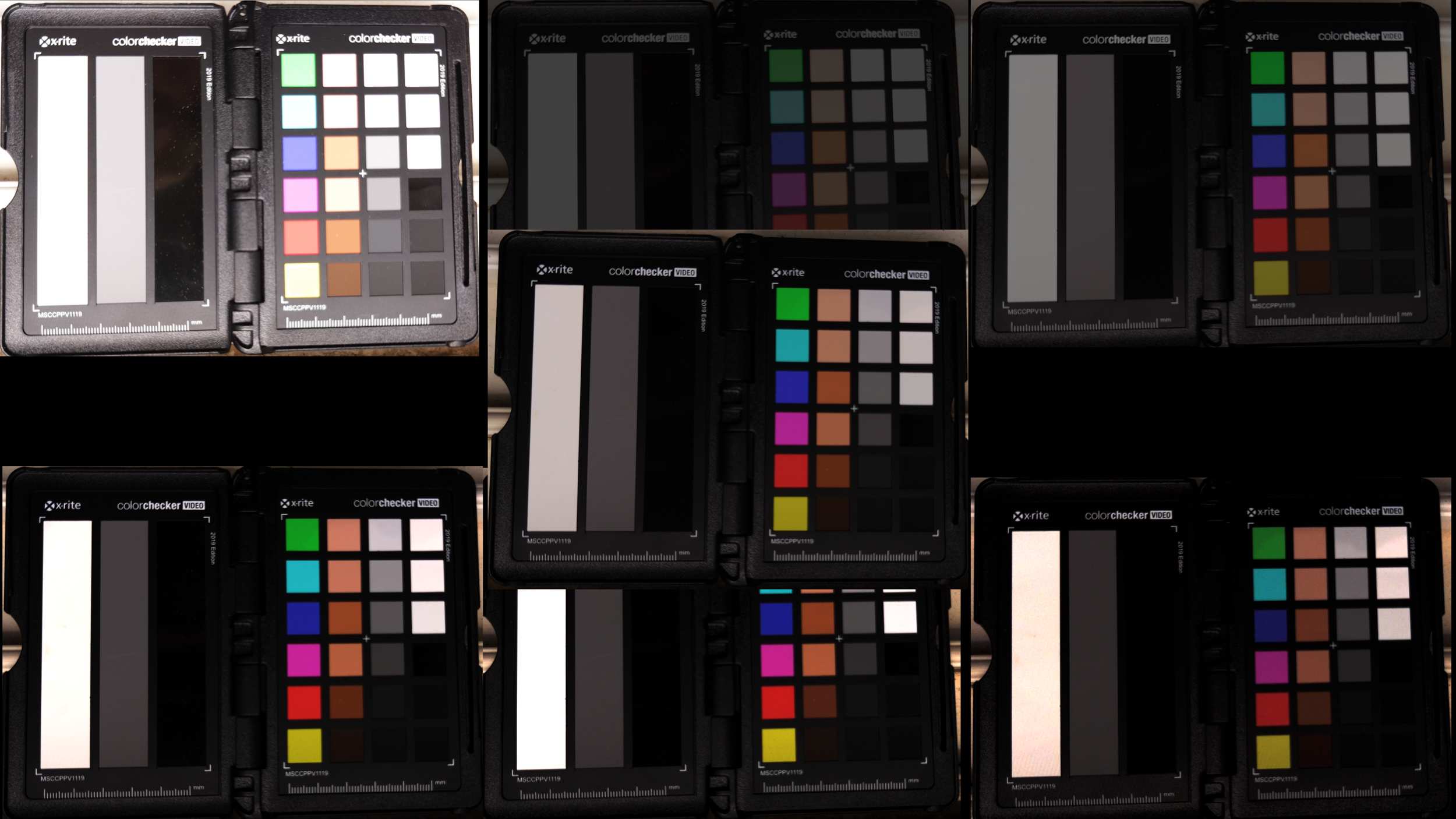
Chart was shot under continuous light, exposure adjusted with shutter time from -3 to +3 EV. Top left +3 ev, top right +1, Middle 0, bottom left -1, bottom right -3.

In the following is the results of the algorithm, Grade for each chart; first node D-Log-M to Linear LUT we created, each exposure normalized with gain (-3ev > 8 gain), end with a Linear to sRGB CST.

You see the algorithm has successfully normalized exposure across the various exposures (except for the chips that were clipped in camera). Similarly the color chips are very consistent and colors true to life.

The following table is a numerical analysis. Reference values are LAB values from chart spec sheet converted to RGB to match picker in Fusion. And bottom rows are % errors vs the reference.

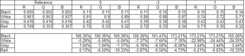
The +3 image looks horrible, but it was very clipped in camera, similarly with +2 ev.

Blacks are about twice what they should be, but are very neutral and quite consistent. Whites are slightly too dark in 0 and -3 ev, +1 ev 23% too dark. Middle Gray and Red, quite accurate.

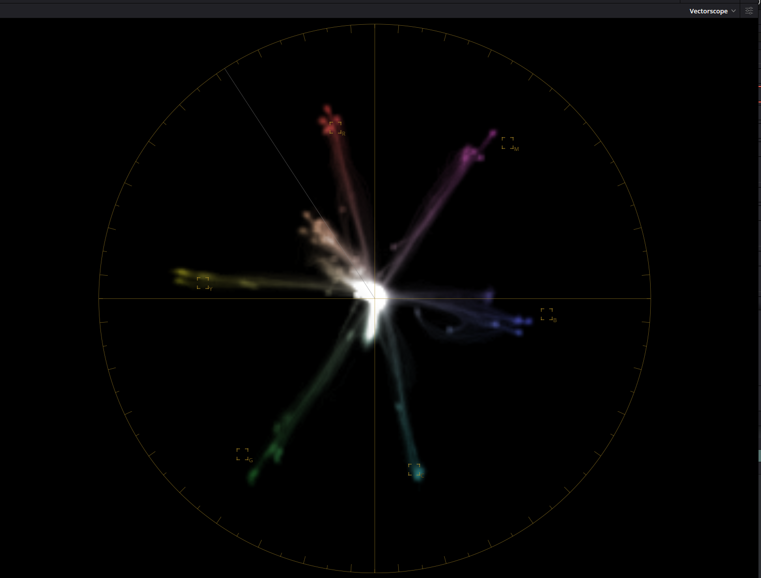
Follows is the vector scope for this image, All chips are grouped quite closely. Blue looks to lack a bit of saturation and be worst grouping. Hue angles very good on red, yellow, cyan and blue.

The same charts with Official DJI to Rec-709 lut, then Rec 709 to Linear CST, Normalization, then Linear to sRGB CST.

Shadows very crushed, the dark gray chips are pure black, and excessive saturation with official lut

And Vector scope, clearly shows excessive saturation, and poor saturation consistency across exposures.

Lut Cube views of algorithm generated lut., doesn't look to have anything crazy going on.

Conclusion:

This genetic algorithm for calculating color space transforms for undocumented color spaces seems to have promise.

There is certainly room for improvement. And with anything it requires good source images to analyze to get good results.

With further development it could be run by any user needing just a test chart with known LAB values and some good light.